After the exercise of building convolutional, RNN, sentence level attention RNN, finally I have come to implement Hierarchical Attention Networks for Document Classification. I’m very thankful to Keras, which make building this project painless. The custom layer is very powerful and flexible to build your custom logic to embed into the existing frame work. Functional API makes the Hierarchical InputLayers very easy to implement.
Please note that all exercises are based on Kaggle’s IMDB dataset.
Text classification using Hierarchical LSTM
Before fully implement Hierarchical attention network, I want to build a Hierarchical LSTM network as a base line. To have it implemented, I have to construct the data input as 3D other than 2D in previous two posts. So the input tensor would be [# of reviews each batch, # of sentences, # of words in each sentence].
tokenizer = Tokenizer(nb_words=MAX_NB_WORDS)
tokenizer.fit_on_texts(texts)

data = np.zeros((len(texts), MAX_SENTS, MAX_SENT_LENGTH), dtype='int32')

for i, sentences in enumerate(reviews):
    for j, sent in enumerate(sentences):
        if j< MAX_SENTS:
            wordTokens = text_to_word_sequence(sent)
            #update 1/10/2017 - bug fixed - set max number of words
            k=0
            for _, word in enumerate(wordTokens):
                if k<MAX_SENT_LENGTH and tokenizer.word_index[word]<MAX_NB_WORDS:
                    data[i,j,k] = tokenizer.word_index[word]
                    k=k+1
After that we can use Keras magic function TimeDistributed to construct the Hierarchical input layers as following. This is what I have learned from this post
embedding_layer = Embedding(len(word_index) + 1,
                            EMBEDDING_DIM,
                            weights=[embedding_matrix],
                            input_length=MAX_SENT_LENGTH,
                            trainable=True)

sentence_input = Input(shape=(MAX_SENT_LENGTH,), dtype='int32')
embedded_sequences = embedding_layer(sentence_input)
l_lstm = Bidirectional(LSTM(100))(embedded_sequences)
sentEncoder = Model(sentence_input, l_lstm)

review_input = Input(shape=(MAX_SENTS,MAX_SENT_LENGTH), dtype='int32')
review_encoder = TimeDistributed(sentEncoder)(review_input)
l_lstm_sent = Bidirectional(LSTM(100))(review_encoder)
preds = Dense(2, activation='softmax')(l_lstm_sent)
model = Model(review_input, preds)

Layer (type)                     Output Shape          Param #     Connected to
====================================================================================================
input_2 (InputLayer)             (None, 15, 100)       0
____________________________________________________________________________________________________
timedistributed_1 (TimeDistribute(None, 15, 200)       8217800     input_2[0][0]
____________________________________________________________________________________________________
bidirectional_2 (Bidirectional)  (None, 200)           240800      timedistributed_1[0][0]
____________________________________________________________________________________________________
dense_1 (Dense)                  (None, 2)             402         bidirectional_2[0][0]
====================================================================================================
Total params: 8459002
____________________________________________________________________________________________________
None
Train on 20000 samples, validate on 5000 samples
Epoch 1/10
20000/20000 [==============================] - 494s - loss: 0.5558 - acc: 0.6976 - val_loss: 0.4443 - val_acc: 0.7962
Epoch 2/10
20000/20000 [==============================] - 494s - loss: 0.3135 - acc: 0.8659 - val_loss: 0.3219 - val_acc: 0.8552
Epoch 3/10
20000/20000 [==============================] - 495s - loss: 0.2319 - acc: 0.9076 - val_loss: 0.2627 - val_acc: 0.8948
Epoch 4/10
20000/20000 [==============================] - 494s - loss: 0.1753 - acc: 0.9323 - val_loss: 0.2784 - val_acc: 0.8920
Epoch 5/10
20000/20000 [==============================] - 495s - loss: 0.1306 - acc: 0.9517 - val_loss: 0.2884 - val_acc: 0.8944
Epoch 6/10
20000/20000 [==============================] - 495s - loss: 0.0901 - acc: 0.9696 - val_loss: 0.3073 - val_acc: 0.8972
Epoch 7/10
20000/20000 [==============================] - 494s - loss: 0.0586 - acc: 0.9796 - val_loss: 0.4159 - val_acc: 0.8874
Epoch 8/10
20000/20000 [==============================] - 495s - loss: 0.0369 - acc: 0.9880 - val_loss: 0.4317 - val_acc: 0.8956
Epoch 9/10
20000/20000 [==============================] - 495s - loss: 0.0233 - acc: 0.9936 - val_loss: 0.4392 - val_acc: 0.8818
Epoch 10/10
20000/20000 [==============================] - 494s - loss: 0.0148 - acc: 0.9960 - val_loss: 0.5817 - val_acc: 0.8840
The performance is slightly worser than previous post at about 89.4%. However, the training time is much faster than one level of LSTM in the second post.
Attention Network
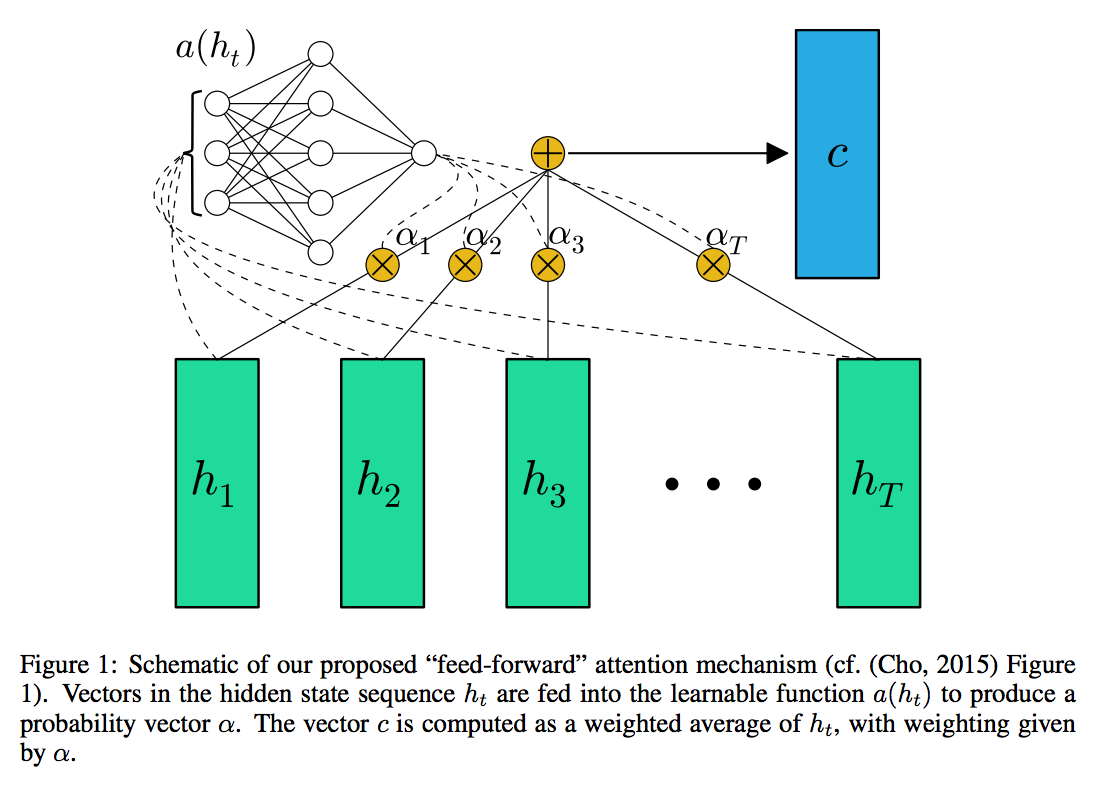
In the following, I am going to implement an attention layer which is well studied in many papers including sequence to sequence learning. Particularly for this text classification task, I have followed the implementation of FEED-FORWARD NETWORKS WITH ATTENTION CAN SOLVE SOME LONG-TERM MEMORY PROBLEMS by Colin Raffel
 |
To implement the attention layer, we need to build a custom Keras layer. You can follow the instruction here
The following code can only strictly run on Theano backend since tensorflow matrix dot product doesn’t behave the same as np.dot. I don’t know how to get a 2D tensor by dot product of 3D tensor of recurrent layer output and 1D tensor of weight.
class AttLayer(Layer):
    def __init__(self, **kwargs):
        self.init = initializations.get('normal')
        #self.input_spec = [InputSpec(ndim=3)]
        super(AttLayer, self).__init__(** kwargs)

    def build(self, input_shape):
        assert len(input_shape)==3
        #self.W = self.init((input_shape[-1],1))
        self.W = self.init((input_shape[-1],))
        #self.input_spec = [InputSpec(shape=input_shape)]
        self.trainable_weights = [self.W]
        super(AttLayer, self).build(input_shape)  # be sure you call this somewhere!

    def call(self, x, mask=None):
        eij = K.tanh(K.dot(x, self.W))

        ai = K.exp(eij)
        weights = ai/K.sum(ai, axis=1).dimshuffle(0,'x')

        weighted_input = x*weights.dimshuffle(0,1,'x')
        return weighted_input.sum(axis=1)

    def get_output_shape_for(self, input_shape):
        return (input_shape[0], input_shape[-1])
Following the paper, Hierarchical Attention Networks for Document Classification. I have also added a dense layer taking the output from GRU before feeding into attention layer. In the following implementation, there’re two layers of attention network built in, one at sentence level and the other at review level.
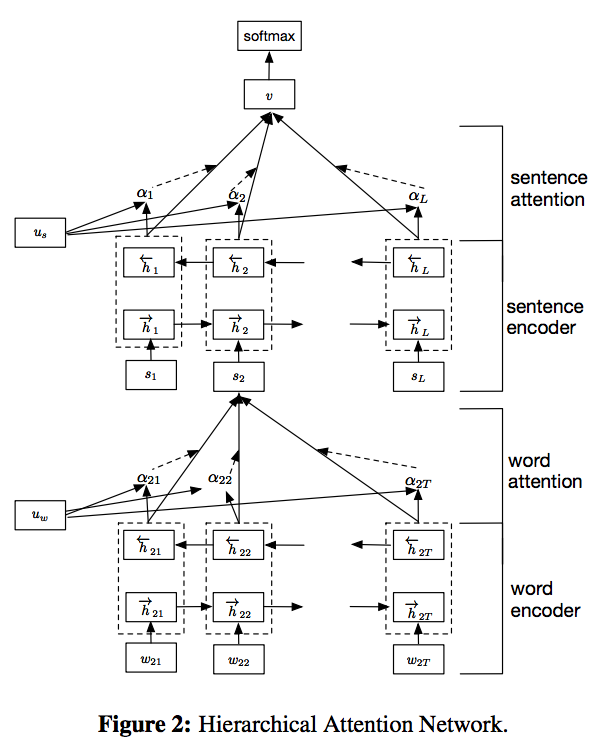 |
sentence_input = Input(shape=(MAX_SENT_LENGTH,), dtype='int32')
embedded_sequences = embedding_layer(sentence_input)
l_lstm = Bidirectional(GRU(100, return_sequences=True))(embedded_sequences)
l_dense = TimeDistributed(Dense(200))(l_lstm)
l_att = AttLayer()(l_dense)
sentEncoder = Model(sentence_input, l_att)

review_input = Input(shape=(MAX_SENTS,MAX_SENT_LENGTH), dtype='int32')
review_encoder = TimeDistributed(sentEncoder)(review_input)
l_lstm_sent = Bidirectional(GRU(100, return_sequences=True))(review_encoder)
l_dense_sent = TimeDistributed(Dense(200))(l_lstm_sent)
l_att_sent = AttLayer()(l_dense_sent)
preds = Dense(2, activation='softmax')(l_att_sent)
model = Model(review_input, preds)

model fitting - Hierachical attention network
____________________________________________________________________________________________________
Layer (type)                     Output Shape          Param #     Connected to
====================================================================================================
input_4 (InputLayer)             (None, 15, 100)       0
____________________________________________________________________________________________________
timedistributed_3 (TimeDistribute(None, 15, 200)       8218000     input_4[0][0]
____________________________________________________________________________________________________
bidirectional_4 (Bidirectional)  (None, 15, 200)       180600      timedistributed_3[0][0]
____________________________________________________________________________________________________
timedistributed_4 (TimeDistribute(None, 15, 200)       40200       bidirectional_4[0][0]
____________________________________________________________________________________________________
attlayer_2 (AttLayer)            (None, 200)           200         timedistributed_4[0][0]
____________________________________________________________________________________________________
dense_4 (Dense)                  (None, 2)             402         attlayer_2[0][0]
====================================================================================================
Total params: 8439402
____________________________________________________________________________________________________
None
Train on 20000 samples, validate on 5000 samples
Epoch 1/10
20000/20000 [==============================] - 441s - loss: 0.5509 - acc: 0.7072 - val_loss: 0.3391 - val_acc: 0.8564
Epoch 2/10
20000/20000 [==============================] - 440s - loss: 0.2972 - acc: 0.8776 - val_loss: 0.2767 - val_acc: 0.8850
Epoch 3/10
20000/20000 [==============================] - 442s - loss: 0.2212 - acc: 0.9141 - val_loss: 0.2670 - val_acc: 0.8898
Epoch 4/10
20000/20000 [==============================] - 440s - loss: 0.1635 - acc: 0.9392 - val_loss: 0.2500 - val_acc: 0.9040
Epoch 5/10
20000/20000 [==============================] - 441s - loss: 0.1183 - acc: 0.9582 - val_loss: 0.2795 - val_acc: 0.9040
Epoch 6/10
20000/20000 [==============================] - 440s - loss: 0.0793 - acc: 0.9721 - val_loss: 0.3198 - val_acc: 0.8924
Epoch 7/10
20000/20000 [==============================] - 441s - loss: 0.0479 - acc: 0.9849 - val_loss: 0.3575 - val_acc: 0.8948
Epoch 8/10
20000/20000 [==============================] - 441s - loss: 0.0279 - acc: 0.9913 - val_loss: 0.3876 - val_acc: 0.8934
Epoch 9/10
20000/20000 [==============================] - 440s - loss: 0.0158 - acc: 0.9954 - val_loss: 0.6058 - val_acc: 0.8838
Epoch 10/10
20000/20000 [==============================] - 440s - loss: 0.0109 - acc: 0.9968 - val_loss: 0.8289 - val_acc: 0.8816
The best performance is pretty much still cap at 90.4%
What has remained to do is deriving attention weights so that we can visualize the importance of words and sentences, which is not hard to do. By using K.function in Keras, we can derive GRU and dense layer output and compute the attention weights on the fly. I will update the post as long as I have it completed.
Full source code is in my repository in github.
Also see the Keras group discussion about this implementation
Conclusion
The result is a bit disappointing. I couldn’t achieve a better accuracy although the training time is much faster, comparing to different approaches from using convolutional, bidirectional RNN, to one level attention network. Maybe the dataset is too small for Hierarchical attention network to be powerful. However, given the potential power of explaining the importance of words and sentences, Hierarchical attention network could have the potential to be the best text classification method. At last, please contact me or comment below if I have made any mistaken in the exercise or anything I can improve. Thank you!
Update - 1/11/2017
Ben on Keras google group nicely pointed out to me where to download emnlp data. So I have used the same code run against Yelp-2013 dataset. I can’t match author’s performance. The one level LSTM attention and Hierarchical attention network can only achieve 65%, while BiLSTM achieves roughly 64%. However, I didn’t follow exactly author’s text preprocessing. I am still using Keras data preprocessing logic that takes top 20,000 or 50,000 tokens, skip the rest and pad remaining with 0. I felt there could be some major improvement in performance if we can do the text processing right, such as replacing time and money to unique tokens and attaching POS information on the sequence etc.
Update - 6/22/2017
Took couple hours and tried to finish the long due attention weight visualization job. The idea is just to do a forward pass. The steps and codes are following:
- Define a K.function and derive GRU or whatever layer output before Attention input
get_layer_output = K.function([model.layers[0].input, K.learning_phase()], [model.layers[2].output])
test_seq = pad_sequences([sequences[index]], maxlen=MAX_SEQUENCE_LENGTH)
out = get_layer_output([test_seq, 0])[0]  # test mode
print(out[0].shape)- Repeat the process in attention weights calculation.
eij = np.tanh(np.dot(out[0], att_w[0]))
ai = np.exp(eij)
weights = ai/np.sum(ai)
weights will be the attention weights, the dimension is 1000 for this program.
- Now you can get what are the top weights of words
K = 10
topKeys = np.argpartition(weights,-K)[-K:]
print topKeys
print test_seq[0][topKeys]
However, the top keywords I am getting are not the desire words I am hopping - some make senses but some don’t. I will continue to investigate when time is allowed. Please message me if you observe something wrong.